QAOA for MaxCut: Solving Real Optimization Problems on Qubits

Everything here is runnable on your own circuit. Try it in the console

The Quantum Approximate Optimization Algorithm is the leading near-term proposal for combinatorial optimization, and MaxCut is its standard model problem. This walkthrough states the construction, runs a real circuit, reports the certified outcome distribution, and sets out honestly where the approach currently stands against classical methods.

MaxCut, and why it stands in for so much

MaxCut asks: given a graph, partition the vertices into two sets so that the number of edges crossing between them is maximised. The problem is NP-hard, and it is APX-hard, meaning no polynomial-time algorithm can approximate it arbitrarily well unless P equals NP.

Its importance is that a large family of practical problems reduces to it. Any quadratic unconstrained binary optimization, or QUBO, maps directly onto an Ising Hamiltonian by the substitution x = (1 - z)/2, and MaxCut is the canonical Ising instance. Circuit partitioning, workload placement, portfolio selection under cardinality constraints, data clustering and spin-glass ground states are all QUBOs, so a method for MaxCut is a method for all of them.

The example here is a four-node ring, vertices 0-1-2-3 joined in a loop. The optimal cut alternates around the ring, cutting all four edges. As bitstrings the two optimal solutions are 0101 and 1010.

The construction

QAOA encodes the objective as a cost Hamiltonian H_C whose ground state is the optimal solution, then prepares an approximation to that ground state with a fixed-depth circuit.

Two layers alternate. The cost layer applies exp(-i gamma H_C), which phases each basis state in proportion to its objective value; for MaxCut this is a ZZ rotation on each edge.

The mixer layer applies exp(-i beta H_B) with H_B the sum of X operators over all qubits, driving transitions between basis states so that amplitude can move toward better solutions. Repeating the pair p times gives 2p parameters, tuned by a classical optimizer.

The construction is motivated by adiabatic quantum computation: as p tends to infinity with appropriately chosen angles, QAOA approaches the adiabatic evolution that provably finds the ground state. At finite p it is a heuristic, and its performance is a numerical question rather than a theorem, which is why simulation carries this field.

A ZZ rotation is implemented as a CNOT, an Rz, and a second CNOT, which is why each edge appears as three gates below. The angles here were tuned for this instance so that the structure is visible in a single layer.

OPENQASM 2.0;
include "qelib1.inc";
qreg q[4];
creg c[4];
h q[0]; h q[1]; h q[2]; h q[3];
// cost layer: a ZZ rotation on each of the four ring edges
cx q[0],q[1]; rz(2.3) q[1]; cx q[0],q[1];
cx q[1],q[2]; rz(2.3) q[2]; cx q[1],q[2];
cx q[2],q[3]; rz(2.3) q[3]; cx q[2],q[3];
cx q[3],q[0]; rz(2.3) q[0]; cx q[3],q[0];
// mixer layer: an Rx rotation on every qubit
rx(0.86) q[0]; rx(0.86) q[1]; rx(0.86) q[2]; rx(0.86) q[3];
measure q -> c;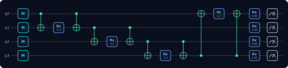

The leading Hadamards place the register in an equal superposition of all sixteen partitions. Each cost-layer edge appears as a pair of CNOTs around a blue Rz. The row of blue Rx boxes near the end is the mixer.

A certified run

The circuit was submitted at 1,000 shots on the exact statevector engine.

counts (top): {"1010": 300, "0101": 259,
               "0011": 81, "1100": 75,
               "0110": 74, "1001": 61,
               "0000": 16, "1111": 29}
error_info:   {"method": "exact statevector",
               "truncation_error": 0.0, "shots": 1000}

The distribution separates into tiers that match the objective values exactly. The two optimal alternating partitions took 559 of 1,000 shots, about 56 percent against the 12.5 percent a uniform distribution would give them.

The four cuts of intermediate quality took most of the remainder. The two worst solutions, 0000 and 1111, which cut no edges at all, drew under 5 percent between them.

A single shallow layer has concentrated measurement on the good cuts by a factor of roughly four and a half. The run carries a public ZCC-v0.1 certificate.

Scaling, and where the cost actually falls

Four qubits fit an exact simulator, so this instance is a demonstration rather than a necessity. The circuit shape scales, and two things change as it does.

The first is that the state leaves statevector range. Ring and near-planar graphs at low p generate entanglement bounded by depth rather than width, so tensor-network engines reach well past 100 qubits: a 100-qubit depth-304 QAOA instance completes in 5.9 seconds on a laptop CPU, fully converged.

Dense graphs at higher p do not compress, and the engine reports a widened bound rather than a fast answer. That report is the signal that the instance has left classical reach. The benchmark is in QAOA at 100 qubits.

The second is that the parameter count grows and the optimisation becomes the dominant cost. A single circuit is not the workload; a 150-iteration SPSA optimisation is 301 circuit evaluations, which is thirty cents in simulation and $352.29 on superconducting hardware.

Using the parameter-shift rule instead multiplies that by the parameter count. The arithmetic is in What does it cost to rent a quantum computer?.

The comparison that matters

QAOA at low p does not currently beat these on instances where both have been evaluated, and there are theoretical obstructions at fixed p on certain graph families. The open question is whether growing p, better angle-finding strategies, or problem-specific mixers change that picture at scales beyond simulation. That is a live research question with no settled answer, and it is worth stating as such rather than resolving it in either direction.

Here is what that looks like on a real instance rather than a toy graph. The same construction is applied to satellite observation tasking at 14 requests, run on the classical engines and on three quantum processors. At this width the true optimum is available by exhaustive search, so every row can be scored against the answer rather than against another approximation.

Run on our engines

Satellite observation tasking at 14 requests, seed 20260902, whose exact optimum is value 32.5128. On 25 September the same instance ran on exact.tpu, a Google TPU, which returned 31.2164 and the smallest gap on the table. Submitted to each kind of compute we offer, on 16 and 25 September 2026 at 500 shots. Every figure below is a real job on the service, priced as any customer would be priced.

Device	Engine	Kind	Qubits	Result	Cost
	mps.quimb.cpu	CPU	14	25.1546, gap 7.36 certificate	$0.0001
	exact.cpu	CPU	14	20.0569, gap 12.46 certificate	$0.0001
	exact.gpu	GPU	14	25.1546, gap 7.36 certificate	$0.0001
	qpu.iqm.garnet	QPU	14	26.8778, gap 5.64 certificate	$1.025
	qpu.rigetti	QPU	14	27.0176, gap 5.49 * certificate	$0.5125
	qpu.iqm.emerald	QPU	14	26.9421, gap 5.57 certificate	$1.100
	exact.tpu	TPU	14	31.2164, gap 1.30 certificate•best outcome	$0.0776
	neural.tpu	TPU	—	the tasking QUBO is diagonal, which is not the shape a neural ansatz is for	—

* The Rigetti row is a separate sample of ours on this same instance, with the QAOA angles re-optimised for it. The steps are in the docs.

A note on the hardware certificates: they state Hellinger fidelity against the exact distribution. For an optimisation circuit that distribution is spread across many outcomes rather than concentrated on one, so the figure is low by construction and is not a measure of whether the device found a good answer. The result column above is.

The same problem is yours to run: every instance here is seeded, so it rebuilds exactly. Open the console and a cost estimate is free before anything executes.

No row reaches the optimum of 32.5128, and the gaps are the honest output of the method at this depth. The classical engines run the identical circuit for a hundredth of a cent, which is the comparison the section above argues for. The question is never whether a QPU beats exhaustive search, but whether it beats the cheapest thing that solves the same instance. The sector write-up is on space and satellites.

The same algorithm on a different industry, because one instance is an anecdote. This is a 12-asset portfolio choosing exactly four holdings, which is MaxCut's structure with a cardinality penalty added, run on three quantum processors and on the classical engines.

Run on our engines

A 12-asset portfolio choosing exactly 4 holdings, seed 20260902, whose provable optimum is 0.199796. On 25 September the same instance ran on exact.tpu, a Google TPU, which found that optimum. Submitted to each kind of compute we offer, on 16 and 25 September 2026 at 500 shots. Every figure below is a real job on the service, priced as any customer would be priced.

Device	Engine	Kind	Qubits	Result	Cost
	mps.quimb.cpu	CPU	12	0.199796, the optimum certificate•best outcome	$0.0001
	exact.cpu	CPU	12	0.247259, beats 97.6% certificate	$0.0001
	exact.gpu	GPU	12	0.251747, beats 96.4% certificate	$0.0001
	qpu.rigetti	QPU	12	0.247730, beats 97.4% * certificate	$0.5125
	qpu.iqm.garnet	QPU	12	0.221427, beats 99.2% certificate	$1.025
	qpu.iqm.emerald	QPU	12	0.245130, beats 98.0% certificate	$1.100
	exact.tpu	TPU	12	0.199796, the optimum certificate	$0.0776
	neural.tpu	TPU	—	the penalised QUBO is diagonal, which is not the shape a neural ansatz is for	—

* The Rigetti row is a separate sample of ours on this same instance, with the QAOA angles re-optimised for it. The steps are in the docs.

A note on the hardware certificates: they state Hellinger fidelity against the exact distribution. For an optimisation circuit that distribution is spread across many outcomes rather than concentrated on one, so the figure is low by construction and is not a measure of whether the device found a good answer. The result column above is.

The same problem is yours to run: every instance here is seeded, so it rebuilds exactly. Open the console and a cost estimate is free before anything executes.

The row to read first is the tensor network, which found the provable optimum of 0.199796 while every quantum processor and both statevector engines landed between 0.221 and 0.252. Note also that the CPU and GPU statevector engines compute the identical distribution, so the gap between those two rows contains no physics at all, and it is roughly half the spread across the whole table. That is the size of the noise floor any claim of quantum advantage on this problem has to clear. The full instance and its penalty construction are on finance and trading.

Running it

Select QAOA MaxCut in the console and run it. Sweep the two angles and observe the balance between good and bad cuts shift; this is the tuning loop at the heart of every variational algorithm. Then increase p and watch both the concentration improve and the classical optimisation become harder, which is the central tension of the method.

For the chemistry counterpart of the same variational structure, see the VQE hydrogen walkthrough.